The computing challenge: fit a model to an absorption line

This is an exercise we will do in class. Please don't do it ahead of time -- or, if you MUST do it before class, don't tell me :-)

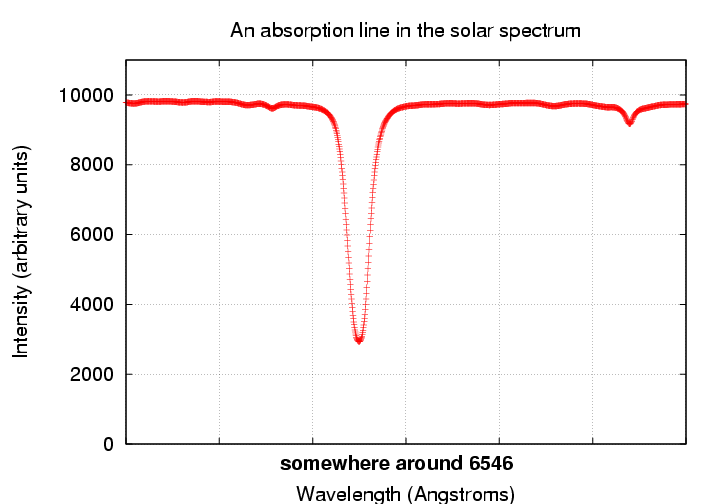
The spectrum of the Sun, like that of most stars, includes many absorption lines. Here's one example:

The measurements on which this graph is based are taken from the BASS2000 website. I have extracted a small section of the data from one spectrum. You can grab this datafile at

http://spiff.rit.edu/classes/ast701/computing/spec_closeup.dat The datafile looks like this:


      6545            9779
      6545.002        9777
      6545.004        9776
      6545.006        9775

where

col 1: wavelength in Angstroms
col 2: intensity of light, in arbitary linear units


   Task 1:  Download the datafile to your computer
            and make a simple plot that resembles the 
            one above.

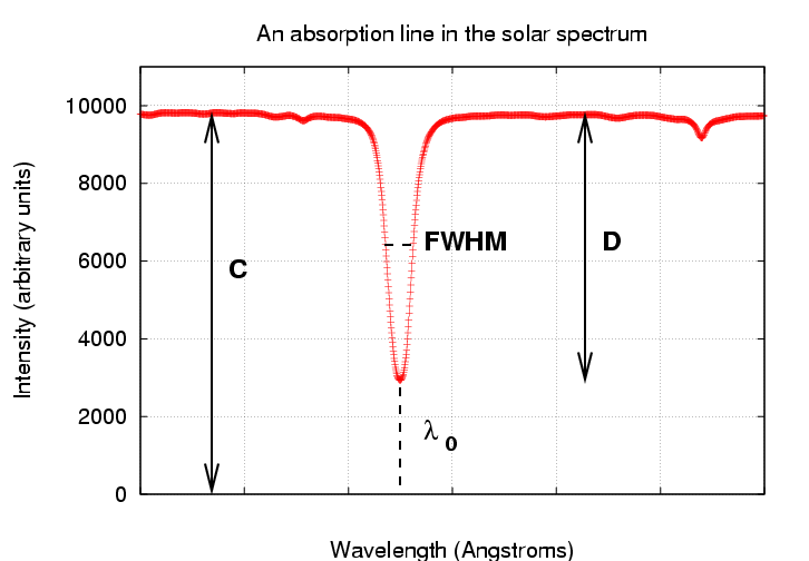
We can describe this line quantitatively with 4 parameters:


   Task 2:  Look at your plot of the data to 
            estimate each of the four parameters by eye.
            Write them down.


   Task 3:  Using your estimates for the parameters,
            generate a model dataset.
            Create a new plot which shows both
            the data and your model.

One way to describe the degree to which some model fits a dataset is to calculate a quantity which is usually called the "chi-squared" statistic.


   Task 4:  Calculate the value of chi-squared
            using your model.
            Use only measurements between
            6546.12 and 6546.38 Angstroms.
            You may assume that the uncertainty in 
            each measurement of intensity is 0.5 units,
            and the uncertainty in each measurement
            of wavelength is negligible.

The chi-squared value, by itself, doesn't tell you all that much about the match between data and model. In order to see if the match is good, you need to do a little extra work.

First, compute the number of degrees of freedom in the problem:

Next, compute the reduced chi-squared statistic like so:

For situations in which the number of degrees of freedom is large, the value of the reduced chi-squared statistic ought to be close to 1.0 .... if

the model is a good representation of the underlying physical phenomenon
the model's parameters have been accurately estimated
the uncertainties are accurately estimated
the errors in the measurements are normally distributed


   Task 5:  Calculate the value of the reduced chi-squared
            statistic using your model.
            Is it close to 1?
            If not, why not?  Which of the possibilities
            listed above is most likely?

One possibility here is that your eyeball estimates of the parameters aren't very good. Is it possible to do better? Yes, probably. How could you do a better job? Is it possible to do a "best" job, in fact?


   Task 6:  Derive better values for the
            4 parameters in your model.
            Explain how you did it.
            Use the improved parameters
            to compute the reduced chi-squared
            statistic again.
            What is it?  What can you conclude?

For more information

Interested in stellar spectra? Consider these nice sources:
- The STELIB library has digital spectra for many stars.
- BASS2000 contains a wealth of information on the sun.
- Spectrophotometric Atlas of Standard Stellar Spectra by Pickles (ApJS, 59, 33, 1985) is a standard source for the spectra of stars. There's a convenient catalog of the spectra in the Vizier system.

This page maintained by Michael Richmond. Last modified Sep 11, 2008.