 Copyright © Michael Richmond.
This work is licensed under a Creative Commons License.
Copyright © Michael Richmond.
This work is licensed under a Creative Commons License.
|
Why should we study radio waves?
This telegram provides one good reason:
to look for extraterrestrials on interstellar comets!
|
Disclaimer -- I'm not a radio astronomer, so it's possible that the next few lectures may contain some mistakes. Please do read some of the references by real experts listed in the 'For more information' section at the end of this document.
The radio, with its much longer wavelengths and much lower energies, differs greatly from the optical or X-ray regimes. Detectors are based on the wave nature of the radiation, rather than the particle-like behavior of photons at higher energies.
At its most basic level, a radio wave (or any electromagnetic wave) can be described as a travelling, oscillating electric and magnetic field.
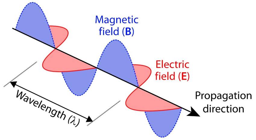
Figure taken from
Verhoeven, AARGnews, 55, 12 (2017)
For today's purposes, only the electric field component is important. If we place a conducting material on the path of such a wave, the passing wave will create an oscillating electric field inside the material; and that field will accelerate charges back and forth through the conductor.
Animation courtesy of
Wikipedia
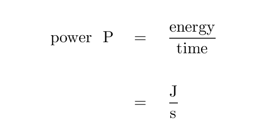
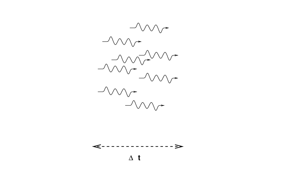
So, a very very very simple radio "telescope" might consist of two long, thin wires, connected by a resistor. We orient the wires in a particular direction, then measure the power dissipated by the resistor.
   Q:   If I place my simple radio telescope's wires
            so that they point East-to-West,
            from which region(s) of the sky
            will it detect sources?
The first radio telescope, operated in the early 1930s, was basically this design.
In the early 1930s, Bell Laboratories wanted to know how practical it would be to send messages across the Atlantic Ocean using radio waves (instead of submarine cables). One of their engineers, Karl Jansky, designed and built a special antenna to study sources of noise in the atmosphere near a wavelength of 14.5 meters. The antenna had two wings, each one wavelength long, mounted on a set of wheels; the entire device would rotate every 20 minutes to scan the sky.
Image courtesy of
NRAO
This telescope could provide only limited information on the direction of the signals it received: it could determine the azimuth, but not the altitude. Jansky connected the receiver to a chart recorder and measured the signal over several days. He saw a clear pattern: one strong source which appeared only during half of each 24-hour period.
(Remember, the telescope is rotating every 20 minutes, so a celestial source will appear as a bump which recurs three times each hour).
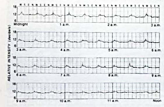
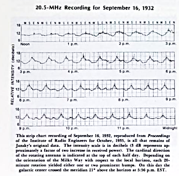
Figure taken from
Sullivan, Sky and Telescope 56, 101 (Aug 1978)
Moreover, Jansky noticed that the signal did not recur with a period of exactly 24 hours; instead, the peak time of the signal drifted slowly over a period of weeks and months.
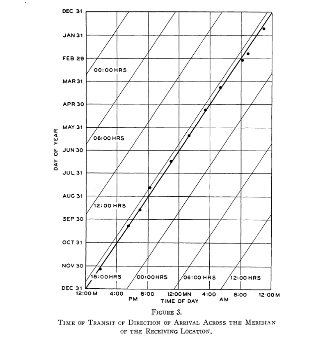
Figure 3 taken from
Jansky, Popular Astronomy, 41, 548 (1933)
  Q:  What is the size of this drift in time?  Express it in both

           a) how long does it take for the signal to drift by 2 hours?

           b) how many minutes does it drift per day?
The amplitude of this drift was about 4 minutes per day ... which is the difference between the solar and sidereal days.
   Q:  What is a solar day?

   Q:  What is a sidereal day?

   Q:  Why are they different?
This was a clear indication that the source of these radio waves was extraterrestrial. In fact, Jansky was able to suggest a specific celestial object as the source of the waves.
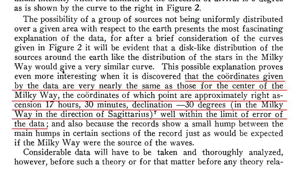
Text taken from "Discussion" section of
Jansky, Popular Astronomy, 41, 548 (1933)
Many years later, Woodruff Sullivan used Jansky's measurements to create a map of the sky. As you can see, even though the center of the Milky Way was slightly outside the region of Jansky's scans, it is clearly a strong candidate to be the source.
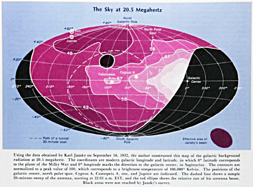
Figure taken from
Sullivan, Sky and Telescope 56, 101 (Aug 1978)
Jansky was intrigued by this evidence of radio waves from celestial sources, and suggested that bigger, better radio telescopes be constructed to study them. Unfortunately, Bell Labs was not interested; they had learned the answer to their question about transatlantic radio communication ("naturally occurring sources of static are not a big problem"), and moved on. Jansky had to stop his research.
But several years later, one of the readers of Jansky's work decided to carry on his work. A young engineer named Grote Reber, who had applied to work at Bell Labs but was not hired, built a very different sort of telescope in the back yard of his home in Wheaton, Illinois. His design used metal panels arranged into a parabolic shape to focus radio waves onto a detector mounted at the end of four support arms.
Image courtesy of
NRAO
Most telescopes used in radio astronomy over the past eighty years have adopted this sort of design: a reflecting dish of parabolic (or other) shape to collect radio waves over a large area, plus a receiver located at the focus of the dish.
Reber, like Jansky, recorded his measurements in a strip-chart format. The figure below shows data he acquired on several nights during 1939. The instrument he used (a micro-ammeter) registered a DECREASE in its reading when radio waves from the sky impinged upon it, so the dips in the graphs below show times (or locations in the sky) when the radio intensity was strong.
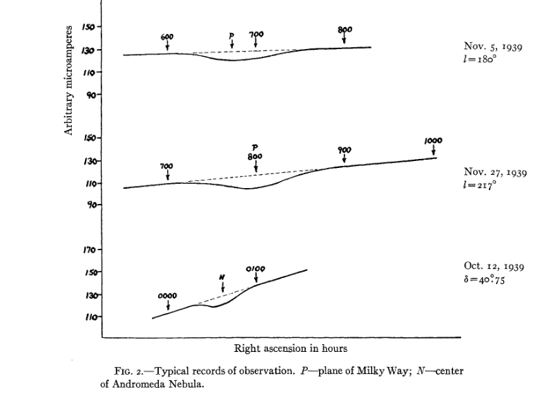
Figure 2 taken from
Reber, ApJ 91, 621 (1940)
Another set of Reber's data, acquired several years later with slightly different equipment (so that now an increase in radio signal corresponds to a RISE in the charts), shows the two strongest sources in the sky approaching each other over a period of several weeks. They are the galactic plane (marked "P", to the left) and the Sun (marked "S", to the right). The celestial signals are both broad, rising and falling gradually as the Earth's rotation brings them into and out of the telescope's field of view. The sharp, short spikes are due to noise from passing automobiles and other terrestrial contaminants (Reber had to work at night to avoid the bulk of automotive interference).
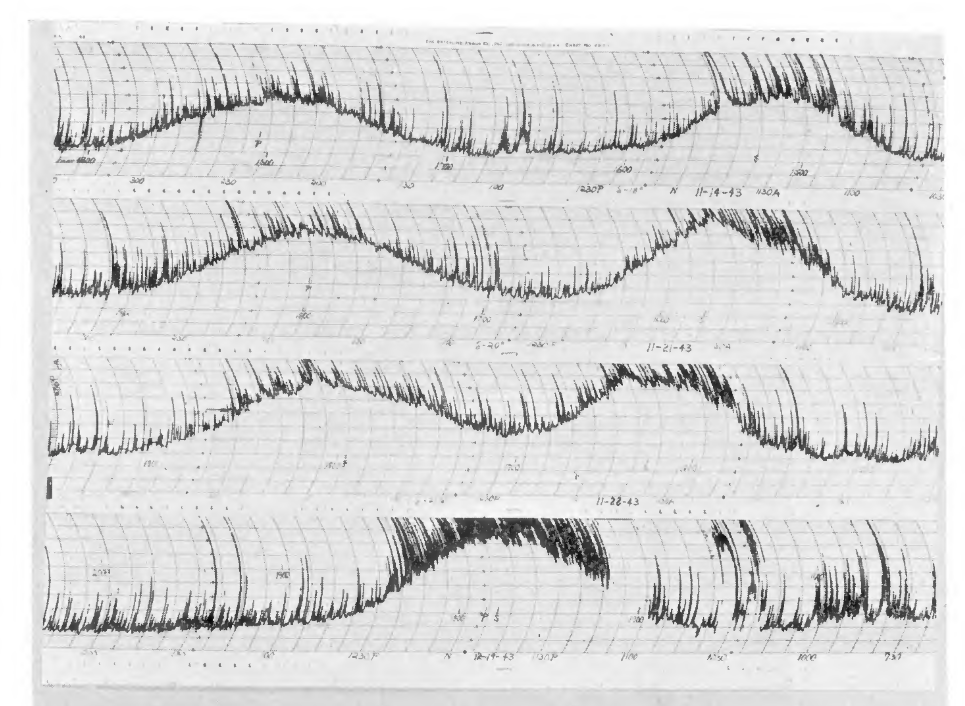
Figure 3 taken from
Reber, ApJ 100, 279 (1944)
Over several years, Reber was able to create a map of the strength of radio emissions at a frequency of about 160 MHz = 1.87 meters. The version shown below has coordinates of Right Ascension (running backwards from 2:00 at left to 14:00 at right) and Declination.
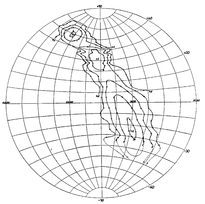
Figure 4a taken from
Reber, ApJ 100, 279 (1944)
  Q:  Can you identify the sources of the three bright spots in this map?

         (Hint: try the desktop version of  Aladin  with the Planck radio survey)
The very simplest sort of radio telescope, like Jansky's, does this job by itself: passing radio waves induce currents to flow through long wires, which can then be measured with instruments. Some modern radio telescopes are designed in the same way -- for example, the UTR shown below.
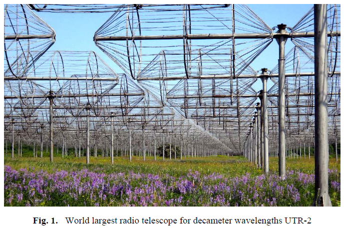
Image courtesy of
Victor Herraro's blog
But many radio telescopes have a dish to collect and focus the radio waves. How are those concentrated waves turned into electrical signals? The answer is via devices called feeds, which are basically little antennae placed at the focus of the dish. The picture below shows two feeds placed near the focus of one dish in the VLA.
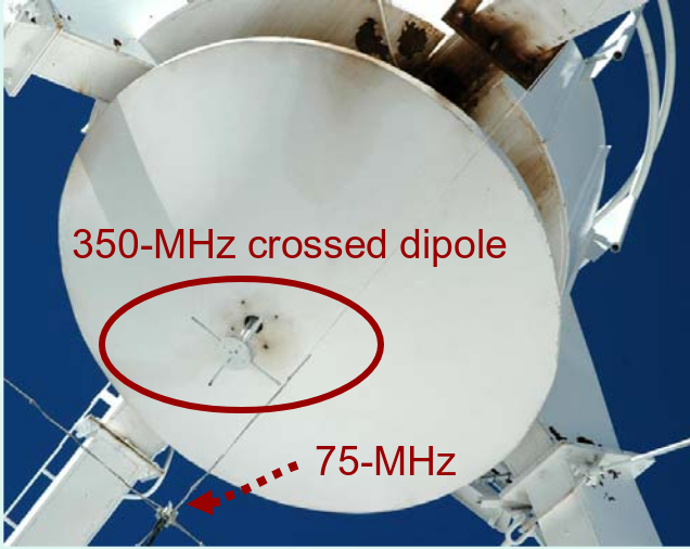
Image courtesy of
Radio Antennas, Feed Horns, and Front-End Receivers
Below are a set of feeds that provide sensitivity at a number of wavelengths.
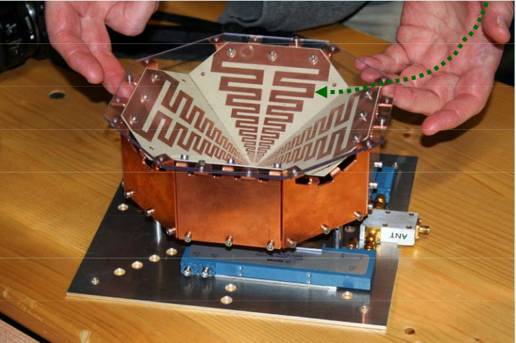
Image courtesy of
Radio Antennas, Feed Horns, and Front-End Receivers
Sometimes, a feedhorn is placed at the focus to improve the connection between waves and feed.
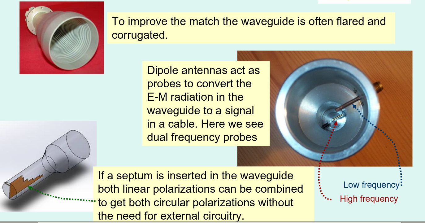
Image courtesy of
Radio Antennas, Feed Horns, and Front-End Receivers
Let's take a look at some of the jargon used by radio astronomers. To me (an optical astronomer), some of the units and terms used to describe observations seem unfamiliar.
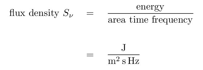
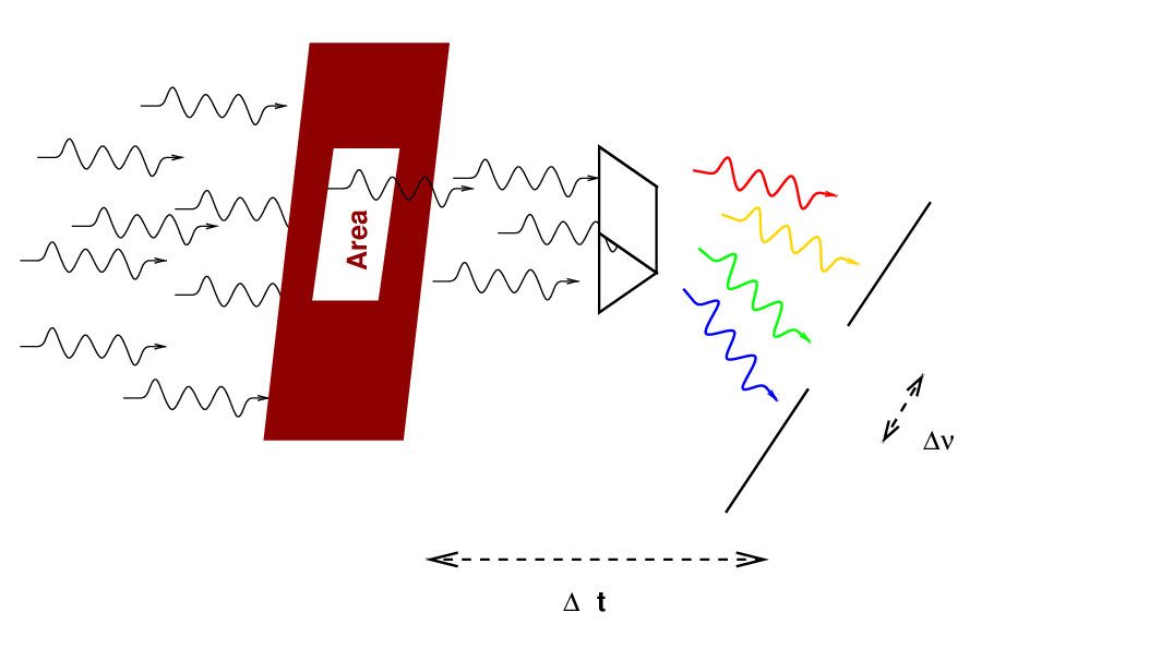
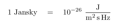
Radio astronomers often measure flux density in units of Janskies. Note that since most radio sources produce very small fluxes at typical frequencies, the definition of 1 Jansky includes a whopper of a coefficient.
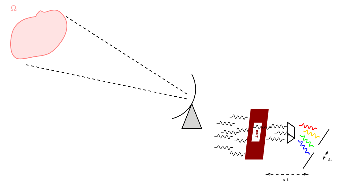
The solid angle of a small patch of sky of angular radius θ is simply
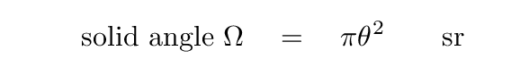
        A steradian is a very large angular area: the entire sky
        contains only 4 π steradians.  Most radio sources,
        and radio beams, are teeny fractions of a steradian.

        The Full Moon has an angular radius of 0.25 degrees.
        What is its angular area in steradians?
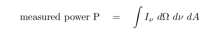
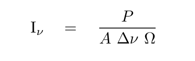
Now, note that a radio telescope may actually measure the power it receives; but we can express that power as an integral over several variables: solid angle, frequency, and collecting area.
Suppose that a star emits radiation with some luminosity L. The flux we measure from that star depends on its distance from us.
For example, the Sun has a luminosity of about L = 3.8 x 1026 Watts.
  Q:  What is the flux from the Sun at a distance of 1 AU?

  Q:  What is the flux from the Sun at a distance of 10 AU?
Definitely not the same. The solar flux decreases with distance from the Sun. Hence the reason probes to the outer solar system need nuclear power.
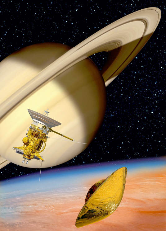
Image courtesy of
ESA
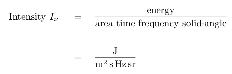
But what about the radio astronomer's quantity called intensity Iν; does the intensity of the Sun change with distance?
If we approximate the Sun as a blackbody of temperature 5600 Kelvin, then one can compute the amount of energy which is radiated within any particular range of frequencies. Let's pick a central frequency of ν = 1 GHz and a bandwidth dν = 0.1 GHz. In that case, the solar luminosity within this narrow band of radio frequencies is about 3.3 gigawatts, and if we divide this luminosity by the bandwidth, we end up with a "luminosity-per-unit-wavelength" which is roughly
In order to compute the intensity Iν, we need to know the solid angle subtended by the Sun in steradians.
The radius of the Sun is about 6.96 x 10⁸ m, and 1 AU is 1.5 x 10¹¹ m, so you can now fill in the table below.
        distance     angular radius       solid angle       intensity
---------------------------------------------------------------------------

       1 AU


      10 AU

---------------------------------------------------------------------------
Note that, in the great majority of cases, we don't know the solid angle subtended by radio sources. That means that in most cases, we can't really compute the intensity properly.
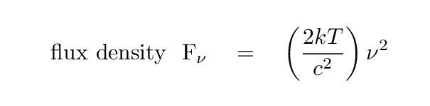
Remember the shape of a blackbody spectrum, when expressed in terms of flux per unit wavelength = flux density? The flux density increases gradually with wavelength until it reaches a peak, then declines very sharply. The logarithmic slope of the spectrum at low frequencies is 2.
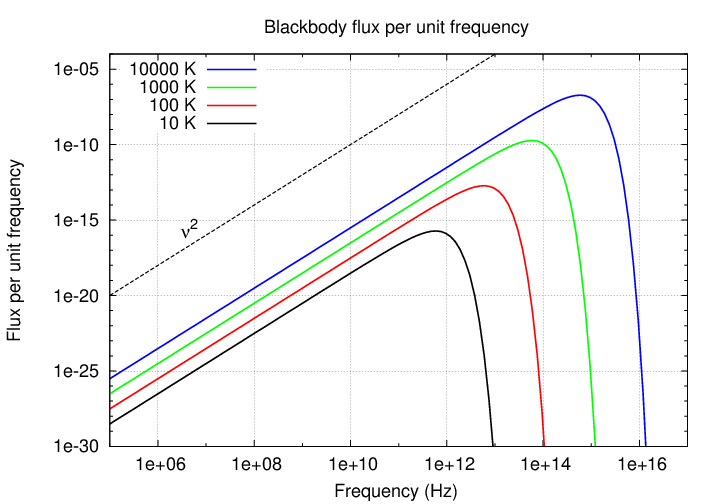
That means that we must be able to express the flux density from a blackbody as some constant X times frequency to the second power.
It can be shown that one way to write this constant X is in terms of temperature and some physical constants, like so:
This looks very much like the expression for intensity; all that is missing is the factor of solid angle. Now, this next step seems to be a bit of a cheat to me, but since steradians, like radians, aren't really units, I guess it's okay. We write that for a blackbody source, the intensity is also a function of frequency-squared.
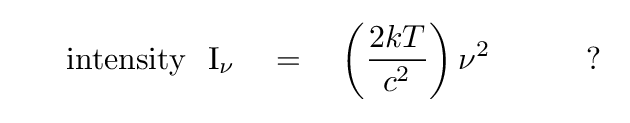
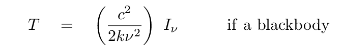
This means that we can turn things around: if we know that we're observing a blackbody, and we are able to compute the intensity properly -- which means knowing the angular size of the source! -- then we can figure out the temperature of the source.
  Q:  Use your value for the intensity of solar radiation at
          a distance of 1 AU, at a frequency of 1 GHz
          (in the table above), to compute the temperature of
          the Sun.
Hey! It works!
So, IF we happen to know that our target is a blackbody, then we can in three steps use radio measurements to compute its temperature.
But even if we don't KNOW that the source is really a blackbody, we can still apply this formula to compute something called the brightness temperature.
What does the brightness temperature mean? Well, if we're lucky, and the source really does emit a Planck spectrum, then the brightness temperature is the temperature of the source. That's the Good News. The Bad News is that if the source is NOT blackbody, then the brightness temperature has no physical meaning at all.
But wait -- there's more Bad News. In order for us to interpret the brightness temperature correctly, we need to know the solid angle subtended by the source. But what if the angular size of the source is unknown?
Well, in that case, the measurement we make will depend upon both the unknown size of the object, and the size of our telescope's beam. The "beam" of a radio telescope is analogous to the PSF of an optical telescope. You will often see a little picture of it in the corner of a radio image, as in the two examples below.
Figure taken from
Sullivan, Sky and Telescope 56, 101 (Aug 1978)
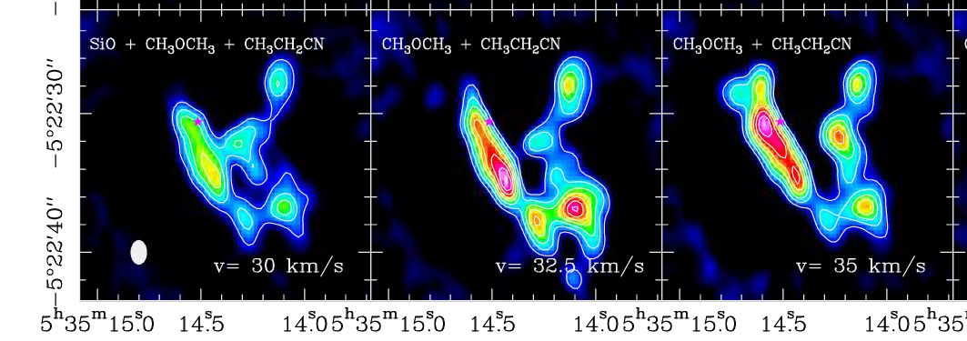
A small portion of Figure 3 taken from
Niederhofer, Humphreys and Goddi, A&A 548, 69 (2012)
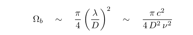
To a first approximation, the beam of a (single dish) radio telescope has an angular size
and therefore subtends a solid angle
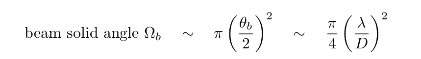
We can write this beam size in terms of frequency, of course:
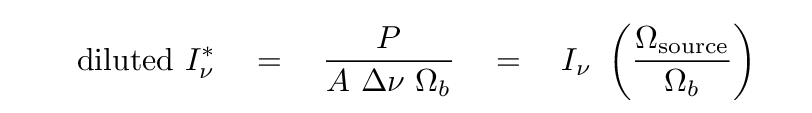
If the beam is larger than the source -- which is usually the case -- then the measured signal is "diluted" by the ratio of the solid angles of the source and beam.
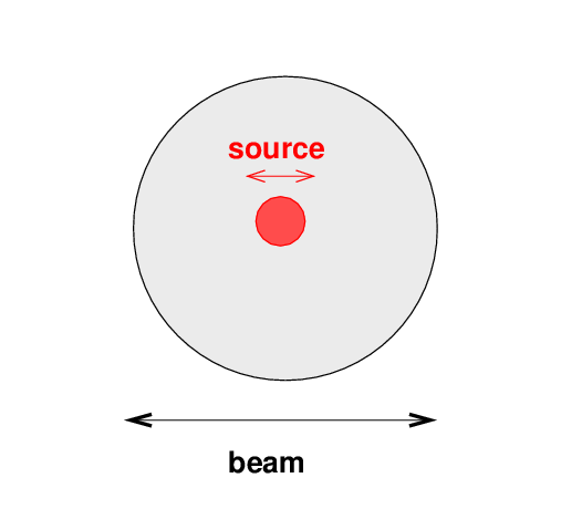
If we use the measured power to compute a measured intensity, that will yield a "diluted" intensity:
And that "diluted intensity" could be used to compute a similarly "diluted" brightness temperature:
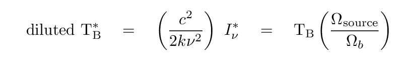
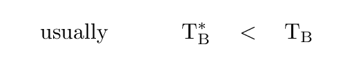
In this case, the true brightness temperature will be larger than the measured, "diluted" version.
Real radio astronomers have a different name for this quantity I've been calling "diluted brightness temperature." They refer to it as antenna temperature T'a, so that
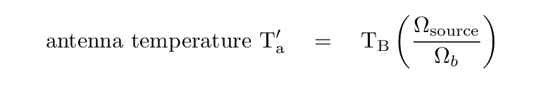
The apostrophe here means that this would be the antenna temperature one would measure if one were above the Earth's atmosphere. The actual antenna temperature might be quite different, but this is as far as I'm going to go into the details.
Antenna temperature is very closely related to the quantity one actually measures with instruments at the focus of a radio dish, so it's important to know how this measured quantity is related to the properties of the source (and one's telescope).
Note that two telescopes of different sizes will still record the same antenna temperature. How? Well, consider two telescopes, with dishes of diameters 1 and 10 meters, operating at a wavelength of λ = 0.3 m.
    dish diam         collecting area          beam            beam
                                              width          solid angle
---------------------------------------------------------------------------

      1  m


     10  m

---------------------------------------------------------------------------
Since the antenna temperature depends on the product of the telescope's collecting area A and beam solid angle Ωb, these two instruments will yield the same antenna temperature.
Let's do one example, just to see the sort of numbers we might deal with in practice. The planet Uranus is sometimes used as a flux calibrator in the radio.
As Weiland et al., ApJS 192, 19 (2011) describe, the brightness temperature of Uranus at a wavelength of 3 cm, or a frequency of 10 GHz, is about 200 K. Suppose we observe the planet with a radio dish of diameter D = 10 m.
  Q:  What is the beam's angular diameter?  What is the beam's solid angle?

  Q:  What is Uranus' angular diameter?  What is Uranus' solid angle?

  Q:  By what factor is Uranus' intensity diluted?

  Q:  What is the antenna temperature we would measure?
Copyright © Michael Richmond.
This work is licensed under a Creative Commons License.