Chandra X-ray data exercise 1

Starting ds9
Playing with Tycho
Using Chandra-Ed Tools: adding up counts
Using Chandra-Ed Tools: making a spectrum
Variations in spectrum across the remnant?
Another way to look for abundance variations

Today is the first of a two-part series of exercises in which you will analyze some X-ray data taken by the Chandra satellite. You can find the list of observations from which our targets will be taken at

Chandra-Ed Observations at rutgers.edu

You can find a local copy of the FITS image we'll be examining today at

Tycho SNR, obsid 115

We'll follow many of the steps and instructions given in X-ray Spectroscopy of Supernova Remnants - ds9 Version, which is a resource listed on Chandra X-ray Center's "Investigating Supernova Remnants" page.

Using ds9

We'll be using SAOImage ds9 to display and analyze Chandra data, so make sure that you can run it on your computer. The program is free and has versions that should run on Windows, Mac OS, and Linux.

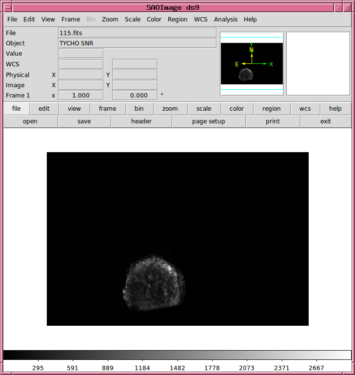
We will use ds9 to download directly the datasets we're going to use in these exercises, rather than copying big datafiles to our hard drives and then opening those local versions. Follow these steps:

run ds9
choose Analysis -> Web Browser ... which should open a new window called "Web". This is a simple mini-browser.
in the Web window, File -> Open URL and enter the URL for the Chandra-Ed Observation archive site:
- http://rinzai.rutgers.edu/archive.html
click on the entry for ObsID = 115, the first line labelled "ACIS Observations of Tycho and Kepler"

This should load the dataset into ds9, and display it in the main ds9 window:

Playing with Tycho

To begin, experiment with the regular ds9 buttons and options to make sure you can

move around to center any desired portion of the image
zoom in and out
figure out the RA and Dec of any area (expressed in decimal degrees or sexigesimal notation)
change the contrast settings of the image

For example, can you set the contrast to a high enough level that you can see the outlines of the individual CCDs on the Chandra focal plane?

In order to enable your ability to create, modify, and delete "regions" of the image, choose Edit -> Region

When you have mastered those tasks, it's time for a bit of calculation. Use the File -> Display Header command to pop up a window with the FITS header of this dataset. Using the information in the header, answer some questions.

Part 1:

How long was the exposure? (Hint: the answer is much longer than 3.2 seconds)
How many arcseconds per pixel? (Hint: look at the CDELT1 and CDELT2 keywords)
Measure the radius of the supernova remnant in arcseconds
Look up the distance to Tycho's SN remnant; not in the FITS header, use ADS Abstract Service to find a paper published in the last 10 years which provides an estimate
Using your measurements of angular radius and distance, compute the linear radius of the remnant
Compute the typical speed of the ejecta, in km/sec

Using Chandra-Ed Tools: adding up counts

Create a region which encloses the entire visible extent of the SN remnant. Now, we'll use one of the tools in the Chandra-Ed toolbox to analyze the properties of the image inside this region. You can access these tools via Analysis -> Chandra-Ed Analysis Tools . The "Overview of Chandra-Ed Analysis Tools" is a good reference -- you might read it if you have questions.

Part 2:

How many counts are inside this region?
Compute the average surface brightness of the entire remnant, in units of counts per pixel

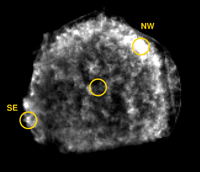
Now, we'll define three areas within the SN remnant: a central region (which is relatively dark), a section of the North-West rim (which is very bright), and a bright knot in the South-East rim. Use the Region command to create a circular region about 10 pixels in radius, and move it to each of these areas in turn to make measurements.

(Hint: it simplifies your life to have only one region at a time. Delete any previous regions before creating a new one).

Measure the surface brightness within each of the three regions.
Express the surface brightness of each region relative to the average surface brightness of the entire remnant.

Using Chandra-Ed Tools: making a spectrum

Remember, one of the features of CCDs in the X-ray regime is that they provide a rough measure of the energy of each photon. We can therefore make a low-resolution spectrum using the information stored in (what looks like) an ordinary X-ray image.

Part 3

Place your circular region of radius 10 pixels over the central portion of the supernova remnant.
Use the Analysis -> Chandra-Ed Analysis Tools -> Quick Energy Spectrum tool to create a quick-and-dirty graph showing the spectrum.
Left-click and drag within the graph to zoom in on the interesting region -- say, from energy 0 - 4000 eV. You can zoom back out to the full graph with right-click.
Identify the energies of the three largest peaks in the spectrum of this region.
Look up the identities of these lines in the X-ray Spectroscopy of Supernova Remnants ds9 Activity
You can examine a list of the spectrum values with File -> List Data option of the graph window. What is the bin size in energy for this spectrum?
Save a copy of the quick-and-dirty spectrum to your computer using the File -> Save Data option. Verify that you can open and read this file.

The "Quick Energy Spectrum" tool is simple and quick, but provides no adjustments. If you want to see a more detailed spectrum, and fit a model to the data at the same time, you can use the Analysis -> Chandra-Ed Analysis Tools -> CIAO/Sherpa Spectral Fit option instead.

Use the Analysis -> Chandra-Ed Analysis Tools -> CIAO/Sherpa Spectral Fit tool to create a detailed spectrum of this region. Choose "Model type" = Brehmsstrahlung, and choose "plot residuals" as well.
Compare this spectrum with that created by the "Quick Energy" tool.
What is the bin size in energy used to create this spectrum?
This tool creates a window which describes the model fit to the data. What was the temperature of the model in this case?
Look at the smooth black line in the graph, which represents the fitted model of brehmsstrahlung radiation. Is it a good fit to this dataset?

Variations in spectrum across the remnant?

Let's do a little scientific investigation. Is this big cloud of gas uniform in its chemical composition, or are there variations in the elemental mix from place to place?

Part 4:

Use a brehmsstrahlung model fit to the data in the central region, and write down the following information:
- fitted temperature of continuum radiation
- elements responsible for all strong emission lines, written in order from strongest to weakest
Repeat for the NW rim region.
Repeat for the SE knot.
Do you see any big differences between these regions?

Another way to look for abundance variations

Let's use another of the Chandra-Ed tools to make a visual check for variations in chemical abundance across the remnant.

Part 5:

Create a region which encloses the entire visible extent of the nebula.
Use Analysis -> Chandra-Ed Analysis Tools -> Energy Filter to display only photons with energies between 1.8 and 1.92 keV. These energies correspond to emission by the K-shell electrons in Silicon atoms.
Use Frame -> Blink to switch between images of all photons, and only those in this range of energies. Do you see any big differences?
Repeat this process for photon energies corresponding to Sulfur, Argon, and Iron K-shell electrons.
Do you see any portions of the remnant which are particularly rich in Iron?
Search for a paper published in 2017 which describes an iron-rich knot in Tycho's supernova remnant. Note the authors and journal reference. Does their knot correspond to yours? What do the authors say about this knot?

For more information

Investigating Supernova Remnants has a number of instructional resources to help you start analyzing Chandra data
SAOImage ds9 is a software package for displaying and interacting with astronomical data.