Optical CCD image analysis, day 1

• Starting AstroImageJ
• Grabbing the images
• Playing with the images
• Creating master dark frames
• Creating a master flatfield frame
• Clean those target images!

Today is the first of a two-part series of exercises in which you will analyze some optical CCD data taken by at the RIT Observatory. You can find the images we'll be using at

• http://spiff.rit.edu/classes/ast613/exercise/v404cyg/

The goal today is to convert a series of "raw" CCD images, with all their defects, into a series of "clean" CCD images. We can then measure properties of stars in the "clean" CCD images in our next meeting.

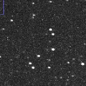
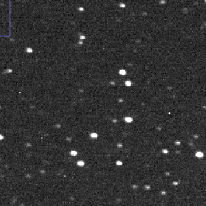
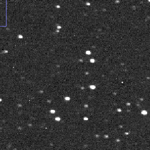
raw	dark-subtracted	dark-subtracted and flat-fielded

Using AstroImageJ

We'll be using AstroImageJ to display and analyze CCD images, so make sure that you can run it on your computer. The program is free and has versions that should run on Windows, Mac OS, and Linux.

One of our former RIT graduate students, Andy Lipnicky, has written some tutorials for using AstroImageJ.

• Andy Lipnicky's guide for AstroImageJ

You might read his guide if you have questions along the way.

Grabbing the raw images

First, you should download copies of the raw FITS images we'll be using to your local computer. There are about 130 images, but each one is pretty small (only 512 x 512 pixels), so the total size of the dataset is only around 68 Megabytes.

First, grab this gzip'ed tar file:

• http://spiff.rit.edu/classes/ast613/exercise/v404cyg/v404cyg_data.tgz

Download it and place it into a new, empty directory (folder) on your computer. Then unpack it. You should find a mixture of images: darks, flats, and target images of V404 Cygni.

Create a new sub-directory (folder) inside this directory full of images. Call this new sub-directory work.

Part 1:

1. How many dark images are there? Do they all have the same exposure time?
2. How many flatfield images are there?
3. How many images of our target, V404 Cyg, are there?
4. Where is this star in the sky? Use SIMBAD or some other tool to look up the RA and Dec. Write them down.
5. Make a finding chart for this star, using Aladin or some other tool. Choose a field of view roughly 15 x 15 arcminutes.

Playing with the images

To begin, experiment with the regular AstroImageJ commands and options to make sure you can

• display an image
• move around to center any desired portion of the image
• zoom in and out
• change the contrast settings of the image
• examine the FITS header of the image

Pick just one of the target images: v404cyg_i-400.fit, which I'll call "target image 400" for short. Below is a picture of this raw image:

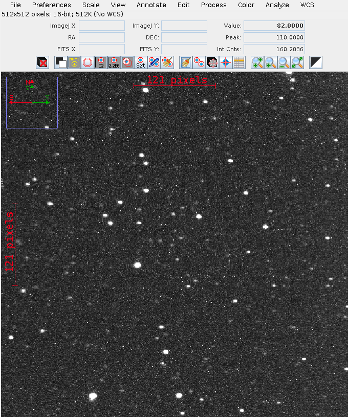
Open this image and use it to answer the following questions.

Part 2:

1. What date was this taken?
2. Which filter was used?
3. How long was the exposure?
4. What is the image orientation? In other words, using the default view, which way is North and which way East?
5. How can you cause AstroImageJ to make the image displayed in the standard orientation of "North up, East left"?
6. How many arcseconds per pixel? Since there are no CDELT1 or CDELT2 keywords in the FITS header, you'll have to figure this out the old fashioned way:
   • Pick two stars which you can identify in both the finding chart and the raw image, and which are reasonably far apart. Label them "A" and "B".
   • Use the finding chart (Aladin) to measure the distance between these two stars in arcseconds
   • Use the raw image (AstroImageJ) to measure the distance between these two stars in pixels
   • Compute the number of arcseconds per pixel. This is sometimes called the "plate scale."

Creating master dark frames

If we take a picture with the shutter closed, our camera SHOULD record an image which is completely empty -- no signal at all. Right? But CCDs don't work that way. Even if no light hits the silicon, electrons can still be knocked free by thermal motions of the atoms.

Let's find out just how large a signal is created this way.

First, create a "master" dark frame from the 20 individual 1-second dark exposures. Open the first image, so that you see a window showing that image. Then, in that's window's "File" menu item, choose Open Image Sequence in new window. Fill in the following menu so that you choose all the images with names like

      dark1-*

Once you have a "stack" of all 20 of these images, you can view each one in turn by dragging the slider at the bottom of the window.

Next, combine all these images into a single, "master" 1-second dark by using Process -> Combine stack slices into single image command; choose the "median" option.

Save the "master" dark as a FITS image with name master_dark1.fits.

Part 3:

1. What is the typical pixel value in this master dark?
2. Use the Analyze -> Histogram option of the little command bar to create a histogram of all pixel values. It may help to specify histogram limits of X Min = 50 and X Max = 100.
3. What is the pixel value at the peak of the histogram?
4. What is the rough Full-Width-at-Half-Maximum of this distribution of pixel values?

There is also a series of 20 dark images with a longer, 20-second exposure time. Use the same steps to create a "master" 20-second dark image, called master_dark20.fits.

4. Use the Analyze -> Histogram option of the little command bar to create a histogram of all pixel values in this longer dark image.
5. What is the pixel value at the peak of the histogram?
6. What is the rough Full-Width-at-Half-Maximum of this distribution of pixel values?
7. How do the pixel values change in dark images when the exposure time increases? Does that make sense?

Creating a master flatfield image

What should happen if we take an image of a blank white, uniformly lit card? We SHOULD see a picture which has the same pixel values everywhere -- a nice, uniform, white (or maybe grey).

But if you take a real picture with a real CCD, attached to a real telescope, you will usually see something quite different. Something which is NOT uniform at all!

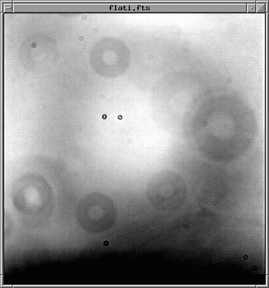
Typically, these "flatfield" images show evidence for several types of defects:

• "donuts" caused by particles of dust on the filters and CCD windows
• large-scale variations due to vignetting by the optics
• small-scale variations due to changes in sensitivity in the silicon or manufacturing process

If we can make a map of these defects, then we can correct for them later. Let's try that with data from this evening. I took pictures of the twilight sky, just after sunset, when it was still too bright to show stars. There is a set of 20 images, all with names like flati-001.fit.

First, we'll need to subtract the "master" dark frame of the appropriate exposure time from each of these raw flatfield images; then, we'll combine them all using a median technique to yield the "master" flatfield image.

Part 4

1. What is the exposure time of these flatfield images?
2. Open a new window to hold a stack of the raw flatfield frames
3. What sort of defects do you see in these images?
4. Choose the Process -> Data Reduction Facility option; two complicated windows will open; close the one called "DP Coordinate Converter"
5. In Science Image Processing,
   • make sure the "Filename Pattern Matching" entry for "Directory" is set to the directory holding your raw images
   • set the "Filename Pattern Matching" entry for "Filename/Pattern" to "flati*", which will match all your raw flatfield images
6. In Bias Subtraction, un-check "enable"
7. In Dark Subtraction, check "enable", and set "Filename/Pattern" to the name of the master dark image you will use
8. In Save Calibrated Images, set the "Sub-dir" entry to work (the directory you created earlier)
9. Click on the big START button

The result should be a set of new, dark-subtracted images inside the new sub-directory you just created.

9. Do the dark-subtracted images look different to your eyes?

It's probably a good idea to close all but one of the image windows you currently have open; the screen is getting crowded.

We can now combine these modified flatfield images to create a "master" flatfield image.

10. Create a new image-sequence window to hold the stack of all 20 dark-subtracted flatfield images, which are in the work sub-directory
11. Combine these via Process -> Combine stack slices into single image again with the "median" option
12. save the resulting file as master_flati.fits, in the same directory as your master dark images (not in the work sub-directory)
13. describe the distribution of pixel values in the master flatfield image, using the "Histogram" command to examine it

Clean those target images!

Okay, we're ready for the big step: we are going to clean the target images. Our procedure will be equivalent to these mathematical steps:

       Step 1:      subtract appropriate master dark

       Step 2:      divide by a normalized version of master flat

We could also write that, on a pixel-by-pixel basis, we will do this:

                              raw(i,j) - master_dark(i,j)
  clean pixel (i,j)  =   [ --------------------------------- ]  * FLATMEAN
                                   master_flat(i,j)

where FLATMEAN is the mean pixel value in the master flatfield image.

The quick and easy way to do this in AstroImageJ is to use the Process -> Data Reduction Facility again. Create a new window to hold a stack of images: the raw target images of V404 Cyg.

Part 5:

1. Choose the target images to process -- all 70 of the images with names like "v404cyg_i-*"
2. Open a new window and read into a stack these raw images
3. Use the slider bar at the bottom of the stack window to view the images, one after another. Do the stars appear to move? Do the hot pixels appear to move?
4. Open the Process -> Data Reduction Facility window, but close the "Coordinate Converter" window
5. Set the Science Image Processing filename to a pattern that matches these raw target images
6. Enable dark subtraction, and enter the name of the appropriate master dark image
7. Enable flat division, and enter the name of the appropriate master flatfield image
8. set the Save Calibrated Images entry to save your clean images in the work sub-directory
9. hit the big START button

The result should be that a set of nice-looking images appears in your work sub-directory. These images should be mostly free of hot pixels, and mostly free of obvious flat-field image defects.

If your images still look crummy, check with the instructor.

Measure the clean images

Okay, you have a set of clean images showing V404 Cyg and a bunch of other stars. Good! We'll deal with photometry next time, so for now, just measure some image properties and get ready for the science.

Part 6:

1. What is the typical pixel value in the star-free background regions of your clean images?
2. What is the source of this "background sky" light?
3. Which star is V404 Cyg? Make a chart and label on it V404 Cyg and 3 stars of similar brightness; call those comparison stars "A", "B" and "C".
4. Measure the peak pixel value in V404 Cyg. What is it?
5. Use the Analyze -> Plot Seeing Profile tool to create a radial profile around V404 Cyg.
6. What is the FWHM of this image in pixels? What is the FWHM in arcseconds?
7. How does the FWHM of comparison stars compare to that of V404 Cyg?
8. Examine all the images in your set. Does the FWHM change much from image to image?

For more information

• AstroImageJ home page
  • Having troubles using AstroImageJ under Mac OS? Lexi Irwin collected some tips and tricks for Mac OS users
• These lectures from another course may provide some useful info about typical CCD processing.
  • making and using median dark images
  • making and using flatfield images
  • cleaning raw CCD images

Copyright © Michael Richmond. This work is licensed under a Creative Commons License.