Many scientists use LaTeX (or its ancestor TeX) to write their journal articles, books, and reports. LaTeX is not an ordinary word processing program like Microsoft Word; instead, it's a typesetting program. There's another difference as well. Most word processors you may have used are interactive and run in a WYSIWYG (What You See Is What You Get) mode: as you type characters, you see the results immediately on your screen. TeX, on the other hand, was originally designed to run non-interactively, taking a pre-written text file as input and creating a nice typeset document as output.
In other words, when you are working with LaTeX, you'll probably follow this pattern:
If all you want is the template for the lab report you'll write in this class, you should read this page and looks at its links.
Once you have installed LaTeX properly on your computer, you can try to run it to turn an input file into a typeset document. I'll show you a few very simple examples, just to give you an idea for how the process works.
Here's a very simple input text file.
\documentclass[twocolumn,11pt]{article}
\setlength{\textheight}{9truein}
\setlength{\topmargin}{-0.8truein}
\setlength{\parindent}{0pt}
\setlength{\parskip}{10pt}
\setlength{\columnsep}{.5in}
\newcommand{\beq}{\begin{equation}}
\newcommand{\eeq}{\end{equation}}
\begin{document}
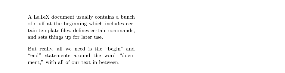
A LaTeX document usually contains a bunch of stuff
at the beginning which includes certain template files,
defines certain commands, and sets things up for later use.
But really, all we need is the ``begin'' and ``end''
statements around the word ``document,'' with all of our
text in between.
\end{document}
This input file has a structure which is common to all LaTeX input files: a bunch of LaTeX commands at the very beginning -- you can recognize them by the backslash characters which start each one -- and then the real text. LaTeX is an example of a "markup language". It breaks the document into pieces, demarcated by the keywords \begin and \end. This very simple example has only one piece: the whole document. Typical documents might have many pieces: an introduction, several chapters, an appendix, a bibliography, and so on. Each piece will have its own pair of \begin and \end markers surrounding it.
Here's the typeset document produced by running LaTeX on the above input file:
LaTeX really shines when it is given the chance to typeset equations. The input format takes some time to learn, but once you know how to use it, watch out! I'll provide just a very simple set of some basic equations as an example; you can find many more detailed guides to typesetting equations in LaTeX in the library and online.
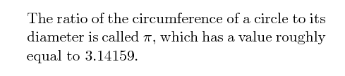
If you want to insert some mathematical language into the body of your text, just surround the math with dollar signs, like this:
    The ratio of the circumference of a circle
    to its diameter is called $\pi$, which has
    a value roughly equal to $3.14159.$
That will yield a paragraph in the document which looks like this:
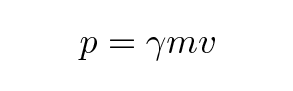
If you want to create an equation which stands alone, set off from the text by some blank space (a "displayed equation"), then the basic idea is to surround the expression by a \begin{equation} and \end{equation}. Inside this region, there are special rules for turning text into typeset material. For example, by default, all letters are printed in italic font, because that's the standard in mathematical work. To print a Greek letter, one must spell out the letter's name, preceded by a backslash. So, for example, this input text
\begin{equation}
p = \gamma m v
\end{equation}
produces this typeset material:
There are LOTS of additional capabilities, but each one involves learning some additional rules. If I want to place the preceding equation into vector form, for example, I can add little arrows over some of the symbols like so:
\begin{equation}
\vec{p} = \gamma m \vec{v}
\end{equation}
and running LaTeX on this input text will result in this output:
I won't bother trying to list all the rules for producing typeset equations. Instead, I'll just show you a few more examples, and let you read about the rest in books or online. Here's a long bit of input text, followed by the typeset output it produces.
\documentclass[twocolumn,11pt]{article}
\setlength{\textheight}{9truein}
\setlength{\topmargin}{-0.8truein}
\setlength{\parindent}{0pt}
\setlength{\parskip}{10pt}
\setlength{\columnsep}{.5in}
\newcommand{\beq}{\begin{equation}}
\newcommand{\eeq}{\end{equation}}
\begin{document}
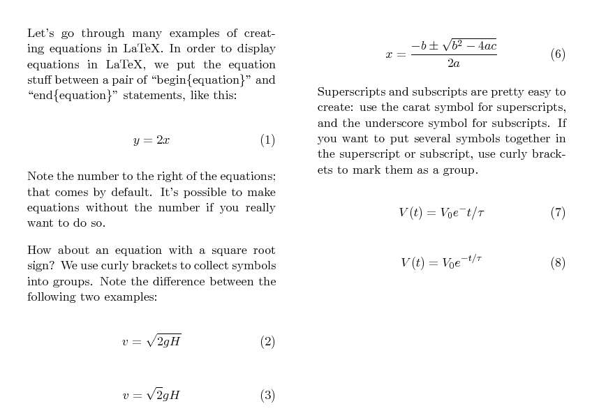
Let's go through many examples of creating equations in
LaTeX. In order to display equations in LaTeX, we
put the equation stuff between a pair of
``begin\{equation\}'' and ``end\{equation\}'' statements,
like this:
\begin{equation}
y = 2x
\end{equation}
Note the number to the right of the equations; that comes
by default. It's possible to make equations
without the number if you really want to do so.
How about an equation with a square root sign?
We use curly brackets to collect symbols into groups.
Note the difference between the following two examples:
\begin{equation}
v = \sqrt{2gH}
\end{equation}
\begin{equation}
v = \sqrt{2} gH
\end{equation}
You can add your own parantheses if you want to
make it very clear to the reader how the symbols
ought to be grouped:
% Look, a comment which is NOT included in the formatted output
\begin{equation}
v = \sqrt{2} (gH)
\end{equation}
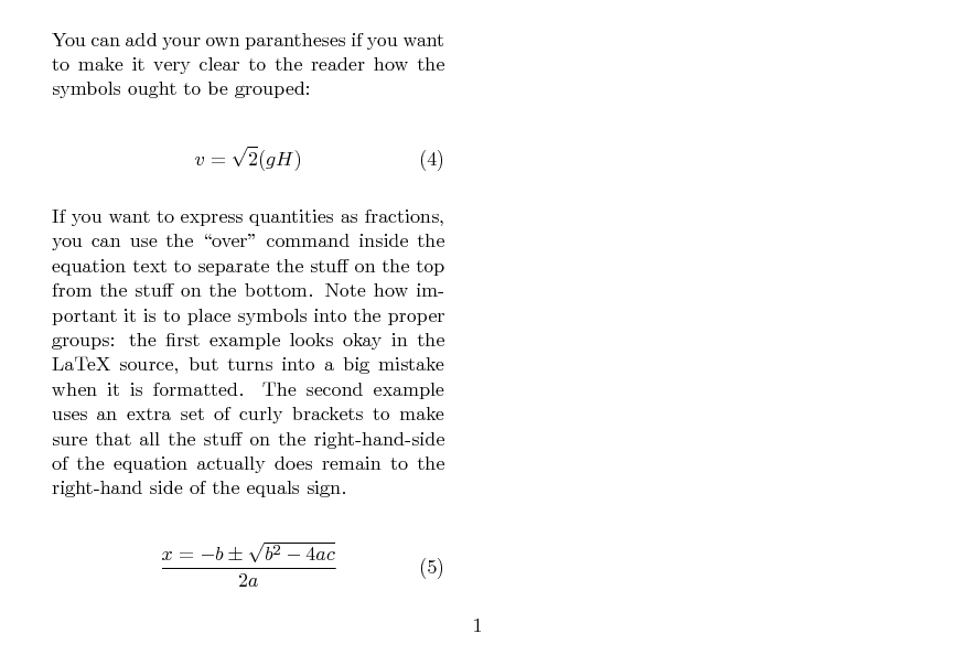
If you want to express quantities as fractions,
you can use the ``over'' command inside the equation
text to separate the stuff on the top from the stuff
on the bottom.
Note how important it is to place symbols
into the proper groups:
the first example looks okay in the LaTeX source,
but turns into a big mistake when it is formatted.
The second example uses an extra set of curly brackets
to make sure that all the stuff on the right-hand-side
of the equation actually does remain to the right-hand
side of the equals sign.
% This is not going to work properly
\begin{equation}
x = {-b \pm \sqrt{b^2 - 4ac}}\over{2a}
\end{equation}
% But this will, thanks to an extra set of curly brackets.
\begin{equation}
x = { {-b \pm \sqrt{b^2 - 4ac}}\over{2a} }
\end{equation}
Superscripts and subscripts are pretty easy to create:
use the carat symbol for superscripts, and the underscore
symbol for subscripts.
If you want to put several symbols together in the superscript
or subscript, use curly brackets to mark them as a group.
% This is not going to work properly
\begin{equation}
V(t) = V_0 e^-t/\tau
\end{equation}
% But this will, thanks to an extra set of curly brackets.
\begin{equation}
V(t) = V_0 e^{-t/\tau}
\end{equation}
\end{document}
Suppose you have a nice picture you'd like to include in your document. Maybe it's a diagram like this:
You can insert the picture into a LaTeX document in many ways, each with its own advantages and disadvantages. One of the simplest ways is to use the \begin{figure} and \end{figure} commands, with several other commands inside that "figure" environment. In order to use this method, you must be sure to add a line like this:
\usepackage{graphicx}
to the long set of special LaTeX commands at the very start of an input file, so that it might look like this ...
\documentclass[twocolumn,11pt]{article}
\setlength{\textheight}{9truein}
\setlength{\topmargin}{-0.8truein}
\setlength{\parindent}{0pt}
\setlength{\parskip}{10pt}
\setlength{\columnsep}{.5in}
\newcommand{\beq}{\begin{equation}}
\newcommand{\eeq}{\end{equation}}
\usepackage{graphicx}
After that, in the main body of the input file, it might be as simple as this:
\begin{figure}
  \includegraphics[scale=0.5]{altaz.eps}
  \caption{The alt-az coordinate system}
\end{figure}
One thing that does make some people confused and upset is the ease with which LaTeX may move your figures around within the surrounding text; there's no guarantee that the picture will sit exactly where you want it to be in the final document, as you'll see from the following example:
\documentclass[twocolumn,11pt]{article}
\setlength{\textheight}{9truein}
\setlength{\topmargin}{-0.8truein}
\setlength{\parindent}{0pt}
\setlength{\parskip}{10pt}
\setlength{\columnsep}{.5in}
\newcommand{\beq}{\begin{equation}}
\newcommand{\eeq}{\end{equation}}
\usepackage{graphicx}
\begin{document}
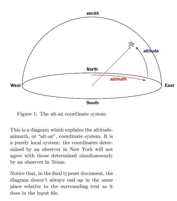
This is a diagram which explains the
altitude-azimuth, or ``alt-az'', coordinate
system. It is a purely local system:
the coordinates determined by an observer
in New York will not agree with those determined
simultaneously by an observer in Texas.
\begin{figure}
\includegraphics[scale=0.5]{altaz.eps}
\caption{The alt-az coordinate system}
\end{figure}
Notice that, in the final typeset document,
the diagram doesn't always end
up in the same place relative to the surrounding
text as it does in the input file.
\end{document}
The typeset document produced looks like this: