
This is a quick example of one way to find the uncertainty in the slope of a line fitted to a dataset; this example shows you how to include uncertainties in one element of the dataset.
Consider the following dataset:
# measurements of current through a material
#
#Current  Volt across     uncert in voltage
# Amps     Volts          Volts
1            4             1.1
2            5             1.1
3            7             1.1
4            9             1.1
5            6             5.1
6            13            1.1
We can use gnuplot to do this work. Other tools -- MATLAB, numpy, Mathematica -- will work, too.
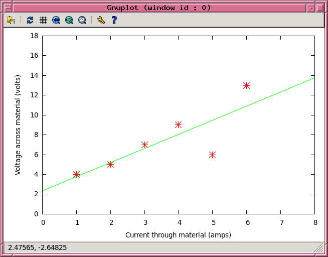
gnuplot> plot [0:8][0:18] 'foo.dat' using 1:2 with points ps 2 pt 3
Uh-oh. Looks like there's one outlier in the dataset. That could cause problems, as we'll see, but it is possible to work around it.
To fit a linear model to the data, y = a + b*x , giving equal weight to all the data, is pretty easy:
gnuplot> f(x) = a + b*x
gnuplot> fit f(x) 'foo.dat' using 1:2 via a, b

               (lots of text scrolls by ...)

********************
After 1 iterations the fit converged.
final sum of squares of residuals : 17.619
rel. change during last iteration : 0

degrees of freedom    (FIT_NDF)                        : 4
rms of residuals      (FIT_STDFIT) = sqrt(WSSR/ndf)    : 2.09875
variance of residuals (reduced chisquare) = WSSR/ndf   : 4.40476

Final set of parameters            Asymptotic Standard Error
=======================            ==========================

a               = 2.33333          +/- 1.954        (83.74%)
b               = 1.42857          +/- 0.5017       (35.12%)


correlation matrix of the fit parameters:

               a      b
a               1.000
b              -0.899  1.000
The slope of the "best-fit" line is about 1.4 volts per amp. But it's not a good fit, really.
gnuplot> plot [0:8][0:18] 'foo.dat' using 1:2 with points ps 2 pt 3, a+b*x
We can do a better job if we use the uncertainty values which are present for each measurement of voltage. They appear in column 3 of the datafile. We can plot them:
gnuplot> plot [0:8][0:18] 'foo.dat' using 1:2:3 with yerrorbars ps 2 pt 3

We can also use them to give WEIGHTS to each of the measurements in the fitting procedure.
gnuplot> g(x) = c + d*x
gnuplot> fit g(x) 'foo.dat' using 1:2:3 via c, d
(lots of text scrolls by ...)
After 1 iterations the fit converged.
final sum of squares of residuals : 1.30837
rel. change during last iteration : -5.09131e-16
degrees of freedom (FIT_NDF) : 4
rms of residuals (FIT_STDFIT) = sqrt(WSSR/ndf) : 0.571921
variance of residuals (reduced chisquare) = WSSR/ndf : 0.327093
Final set of parameters Asymptotic Standard Error
======================= ==========================
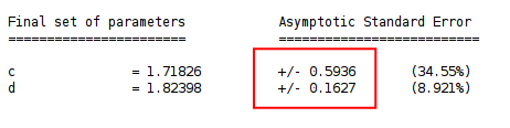
c = 1.71826 +/- 0.5936 (34.55%)
d = 1.82398 +/- 0.1627 (8.921%)
correlation matrix of the fit parameters:
c d
c 1.000
d -0.882 1.000
Aha! Note that the slope is quite different now, as is the intercept. If we plot the new solution as well as the old one, you can see that it is better.

Notice that the fitting routine provides values for each parameter, AND also provides uncertainties in those values.
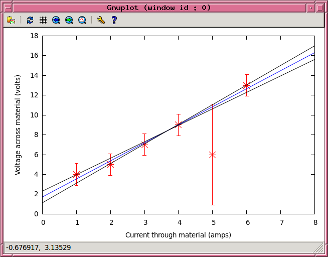
It's easy to tell gnuplot to plot the best-fit line, but also the line corresponding to the largest slope (and smallest intercept), and the line corresponding to the smallest slope (and largest intercept).
gnuplot> plot [0:8][0:18] 'foo.dat' using 1:2:3 with yerrorbars ps 2 pt 3, c + d*x lt 3, (c-0.59)+(d+0.16)*x lt -1, (c+0.59)+(d-0.16)*x lt -1
This page maintained by Michael Richmond. Last modified Sep 26, 2012.